Before the actual placement of low-cost sensors at selected locations within Legerova, Sokolská, Rumunská streets and the surrounding area, these devices were subjected to an initial comparative measurement in outdoor conditions, in order to detect possible malfunctions and measurement deviations.

The raw data measured by low-cost sensors must always be checked because the quality of the measurement is strongly dependent on meteorological conditions, or on the possible interference of various pollutants. After eliminating the detected defects in some pieces, it was found during the comparative measurement that most sensors are able to measure similar concentration trends, however, in absolute values, these concentrations were shifted relative to each other (see news), including detection of a different data shift compared to the reference/control measurement. If these deviations are not identified and an appropriate method is not chosen to correct the raw data, it can lead to a fundamental misinterpretation of the measured values of the pollution level at the locations of interest where the sensors are subsequently placed. Fig. 1 shows an example of a specific situation where, in the case of sensor No. 11 (green color), based on the raw measured data (dashed green line), we could assume that it recorded a lower NO₂ concentration than sensor No. 10 (purple color). However, after back-correcting the data, it was found that sensor No. 11 was actually located in an area with higher NO₂ concentrations than sensor No. 10.
Fig. 1. Example of comparison of raw measured data (dashed line) with data after correction (solid line) for the case of sensors No. 10 (purple color) and No. 11 (green color) located in Sokolská street in Prague.

After detecting deviations in the measurement, it is necessary to choose a suitable method of correction of the raw data measured by the sensors. The first to apply the quite often used method of linear regression, which uses linear relationships between the sensor and the reference measurement to determine the correction coefficient. However, this later turned out to be insufficient, because with the development of time and meteorological changes in the outdoor conditions, non-linear relationships began to appear in the measured data, when the correction treated low and high concentrations with different quality. This led, for example, to a significant underestimation of realistically high concentrations, which is subsequently unsatisfactory when monitoring is installed in heavily loaded locations.

It was therefore necessary to apply a more complex mathematical method that would allow work with non-linear relationships as well, and which would be able to take into account other variables that have a significant effect on the quality of sensor measurements. The best results were finally achieved using the so-called multidimensional adaptive spline regression method, which allows the effect of specific meteorological conditions (temperature and relative air humidity, wind speed, solar radiation intensity and time of day) to be included in the correction equation. This correction method responded much more effectively to low and high concentrations, and therefore did not further underestimate the data.

The results of the correction are shown in Fig. 2, when the sensors were placed at the initial comparative measurement at the same control location (reference station Prague Libuš).
The box plot shows the medians and the range of hourly NO₂ concentrations measured by individual sensors, with raw measured data in blue and back-corrected data in red. It can be seen from the graph that the correction achieved equalization of both the medians and the entire range of measured concentrations for all sensors
Fig. 2. Boxplot showing medians and ranges of 1-hourly NO₂ concentrations originally measured by different sensors (blue color) and back-corrected concentrations by the MARS method (red color).

The same is evident when comparing the course of hourly concentrations. Fig. 3 shows the average hourly concentrations of NO₂ as originally measured by the sensors during the comparative measurement period (sensors at the same control location; highlighted by a blue frame) and subsequently after transmission to the locations of interest within Legerova, Sokolská, Rumunská streets and the surrounding area. Fig. 4 then shows the back-corrected NO₂ concentrations in the same period, which correspond to each other much better than in the original data in the case of the period when the sensors were placed at one control location (highlighted by a blue frame).
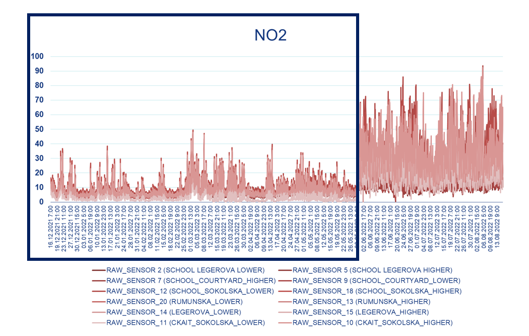Fig. 3. The course of 1-hour NO₂ concentrations (ppb) initially measured by the sensors with the marking of the period when the sensors were at the same location (blue frame) and subsequently after the transfer to the locations of interest.


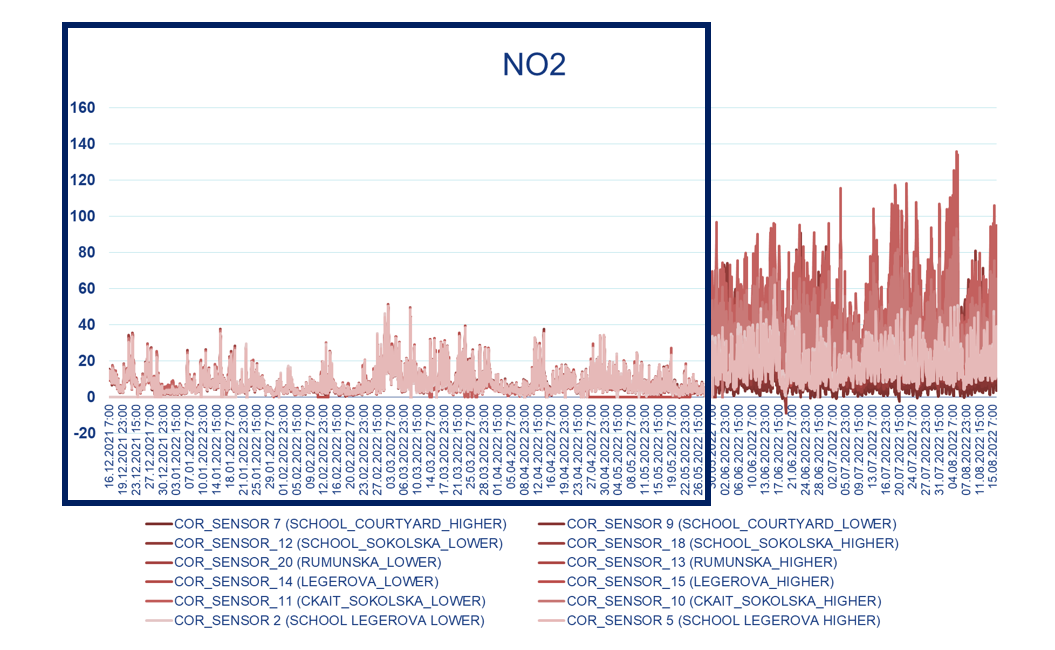Fig. 4. The course of back-corrected 1-hour NO₂ concentrations (ppb) with marking of the period when the sensors were at the same location (blue frame) and subsequently after transfer to the locations of interest.